How to Create a Pivot Table in Microsoft Excel

Are you tired of sifting through endless rows of data in your Microsoft Excel spreadsheets? Do you wish there was an easier way to summarize and analyze large datasets? If so, you're in luck. Pivot Tables are a powerful tool in Microsoft Excel that allow you to easily summarize and analyze large datasets. In this article, we'll show you how to create a Pivot Table in Microsoft Excel and provide you with the knowledge to unlock the full potential of your data.

What are Pivot Tables and Why Do I Need Them?

Pivot Tables are interactive tables that allow you to summarize and analyze large datasets by creating custom views of your data. They're called "Pivot" Tables because you can rotate, or pivot, the data to view it from different angles. With a Pivot Table, you can easily answer questions like "What are the total sales for each region?" or "Which product is the best seller?" By using a Pivot Table, you can quickly and easily summarize and analyze large datasets, making it easier to make informed decisions.

The Benefits of Using Pivot Tables

So why should you use Pivot Tables? Here are just a few benefits:

• Easy data analysis: Pivot Tables make it easy to summarize and analyze large datasets.
• Customizable: You can create custom views of your data by rotating, or pivoting, the data.
• Interactive: Pivot Tables are interactive, so you can easily change the view of your data.
• Time-saving: Pivot Tables save you time by allowing you to quickly summarize and analyze large datasets.

Preparing Your Data for a Pivot Table

Before creating a Pivot Table, it's essential to prepare your data. One common step is to remove duplicates. You can learn how to do this by reading our article on How to remove duplicates in Excel.

Creating a Pivot Table in Microsoft Excel

Now that we've covered the basics of Pivot Tables, let's dive into how to create one in Microsoft Excel.

Step 1: Select Your Data

The first step in creating a Pivot Table is to select your data. To do this:

• Select the cell range that contains the data you want to use in your Pivot Table.
• Make sure the data is in a table format, with each row representing a single record and each column representing a field.

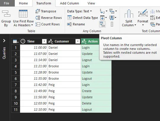
Step 2: Create a Pivot Table

Once you've selected your data, it's time to create a Pivot Table. To do this:

• Go to the "Insert" tab in the ribbon.
• Click on the "PivotTable" button in the "Tables" group.
• Select a cell where you want to place the Pivot Table.
• Click "OK" to create the Pivot Table.

Step 3: Configure the Pivot Table

Once you've created the Pivot Table, it's time to configure it. To do this:

• Drag fields from the "PivotTable Fields" pane to the "Rows", "Columns", and "Values" areas.
• Use the "Filters" area to filter the data in your Pivot Table.

Understanding the Pivot Table Fields Pane

The Pivot Table Fields pane is where you'll configure your Pivot Table. Here's a breakdown of the different areas:

• Rows: This area is where you'll place the fields that you want to use as the rows in your Pivot Table.
• Columns: This area is where you'll place the fields that you want to use as the columns in your Pivot Table.
• Values: This area is where you'll place the fields that you want to use as the values in your Pivot Table.
• Filters: This area is where you'll place the fields that you want to use as filters in your Pivot Table.

You can also use VLOOKUP in combination with pivot tables to look up and retrieve data from other tables. Learn more about how to use VLOOKUP in our article on How to use VLOOKUP in Microsoft Excel.

Customizing Your Pivot Table

Once you've configured your Pivot Table, you can customize it to suit your needs. Here are a few ways to customize your Pivot Table:

• Use the "PivotTable Tools" tab to change the layout and design of your Pivot Table.
• Use the "Analyze" tab to analyze the data in your Pivot Table.
• Use the "Design" tab to change the layout and design of your Pivot Table.

If your data contains text that needs to be converted to numbers, you can learn how to do this by reading our article on How to convert text to number in Excel

Saving and Sharing Your Pivot Table

Once you’ve customized your Pivot Table, you can save your work and share it with others. To save and share:

Save your file: Use Ctrl+S or go to File > Save As and choose your preferred location and file format. Share your file: Send the Excel file via email or share it through cloud services like OneDrive or Google Drive.

Conclusion

Pivot Tables are an essential tool for anyone working with data in Microsoft Excel. They allow you to quickly summarize and analyze large datasets, customize views, and make data-driven decisions efficiently. By following the steps in this guide, you’ll be able to create and customize Pivot Tables like a pro.