How to make a graph in Excel: steps, example and fixes
Make a graph in Excel with a simple sales example. Learn to select data, choose a chart, fix missing labels and correct numbers stored as text.

To make a graph in Excel, select your data including column headings, choose Insert → Recommended Charts, pick a chart and select OK. On Windows, Alt + F1 creates an embedded chart immediately; review the chart type before using it.
These desktop steps follow Microsoft's chart creation instructions for Excel for Microsoft 365, Excel 2024 and Excel 2021. Ribbon labels can vary by platform. In Excel for the web, use the chart controls on Insert; the desktop dialog and shortcuts may differ.
Try this example: monthly sales
Enter this practice dataset in cells A1:B4:
| Month | Sales |
|---|---|
| January | 120 |
| February | 180 |
| March | 150 |
Select A1:B4, then insert a clustered column chart. The intended result has three month labels and bars representing 120, 180 and 150. Give it the title Monthly sales. Use the values above to check that each bar corresponds to its source cell.
Use a column or bar chart to compare categories, a line chart for a sequence over time, or an XY scatter chart when both axes represent numeric measurements. A pie chart uses one series of values with category labels; exclude a total row to avoid plotting it as another slice. See Microsoft's chart data layouts.
Step 1: Select Your Data
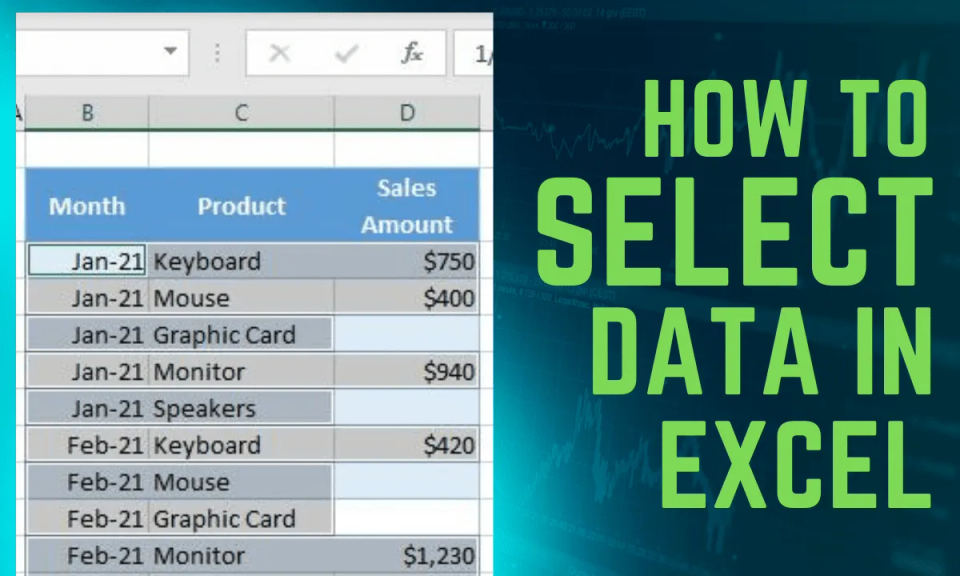
The first step in creating a graph or chart in Excel is to select the data you want to include. This includes headers, labels, and any other relevant data that you want to display in your chart. To select your data, simply click and drag your mouse to highlight the cells that contain the data you want to use.
Tips for Selecting Your Data:
Make sure to include headers and labels to provide context for your data.
Use a consistent format for your data to ensure that Excel can read it correctly.
If you have a large dataset, consider using a table or pivot table to make it easier to manage and select your data.
If you're having trouble formatting your data, you can check out How to convert text to number in Excel, which can provide assistance with data formatting.
Step 2: Insert a Chart

Once you've selected your data, it's time to insert a chart. To do this, go to the Insert tab in the ribbon and click on Recommended Charts. This will open a dialog box that shows you a selection of chart types based on your data.
Choosing a Chart Type
Don't worry if you're not sure what type of chart to use - Excel will suggest some options based on your data. If you prefer to choose a specific type, click on the All Charts tab to view all available chart types.
Popular Chart Types:
Bar chart: Great for comparing data across different categories.
Line chart: Ideal for showing trends and patterns over time.
Pie chart: Perfect for displaying proportions and percentages.
Step 3: Insert and check the result
In the chart dialog, select the preview that fits your data, then select OK. For the practice data, check for exactly three month labels and a single Sales series. If Excel treats the months as separate series, use the troubleshooting steps below before changing colors or labels.
Step 4: Customize Your Chart
Now that you've created your chart, it's time to customize it. To switch the data orientation, select the chart, go to the Chart Design tab, and click Switch Row/Column. To adjust the legend position, select the chart, click the + button on the right side, click the arrow next to Legend, and choose Right.
Customization Options:
Change the chart title: Update the title of your chart to reflect the data you're displaying.
Add data labels: Add labels to your chart to provide more context and information.
Change the chart colors: Update the colors of your chart to match your brand or style.
Step 5: Add Titles and Labels
Add a title to your graph and any necessary data labels to enhance clarity. This will help your audience understand the data you're displaying and what the chart is trying to communicate.
Tips for Adding Titles and Labels:
Keep your title concise and to the point.
Use clear and concise language for your data labels.
Consider adding a subtitle or footnote to provide additional context.
Step 6: Save Your Document
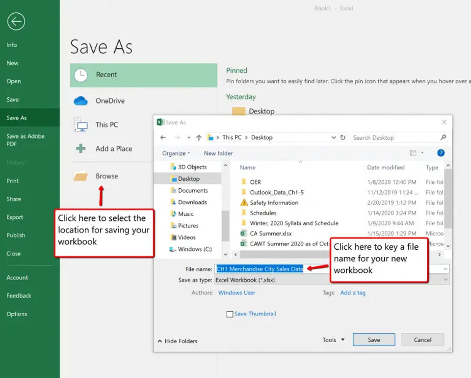
Once you are satisfied with your chart, save your Excel document. This will ensure that all your hard work is saved and you can easily access your chart later.
Tips for Saving Your Document:
Save your document regularly to avoid losing your work.
Consider saving multiple versions of your document to track changes and updates.
Use a clear and descriptive filename to make it easy to identify your document.
Fix common Excel chart problems
The chart is blank or values are missing
Check that your selection includes numeric cells, not just headings. For the example above, select A1:B4. If values are stored as text, follow how to convert text to numbers in Excel, then check the chart again. Keep a copy of source data before changing it.
The months appear as series instead of labels
Select the chart and review Chart Design → Switch Row/Column on desktop Excel. For the example, the months should be category labels and Sales should be one series. If the selection is wrong, use Select Data to review the source range.
The chart includes a total or unrelated column
Review the selected range and exclude summary rows you do not want plotted. Keep a clear header for each column. Microsoft's data selection guide explains continuous and nonadjacent selections.
Recommended Charts is unavailable or unhelpful
Use the chart controls on Insert to choose a specific chart type. On desktop, All Charts in the chart dialog offers more choices. Check Microsoft's platform-specific instructions if your controls differ.
Before sharing
Check that the title describes the data, labels show the correct categories and units are clear. Compare plotted values with the source cells. Keep the workbook so you can revise the data and chart together.
AI-assisted publication. Source checks are not device testing. How we make guides